Decision Tree is a supervised learning algorithm that can be used for both classification and regression. There are two types of Decision tree based on the target variable:

1. Categorical Variable Decision Tree - When target variable is categorical type
2. Continuous Variable Decision Tree - When target variable is continuous type

For example if we need to find out a customer will purchase a house or not than we have a categorical target variable (Yes or No) and if we need to find out how much a customer can pay for a specific house than we have a continuous target variable ( Price of the house).

Assumption of Decision Tree:

1. Feature values are preferred to be categorical if not discretization of continuous variables is required.
2. Training data will be wholly considered as root in the beginning
3. Records are distributed recursively on the basis of attribute value

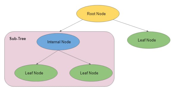
The tree has three type of nodes:

1. Root Node - No incoming edge and zero or more outgoing edge
2. Internal Node - Exactly one incoming edge and two or more outgoing edge
3. Leaf or Terminal Node - Exactly one incoming edge and no outgoing edge

Before going ahead lets look into some terminologies:

1. Splitting - Dividing a node into one or more sub-nodes
2. Pruning - Removing nodes to reduce the size of decision tree
3. Branch / SubTree - Subsection of decision tree
4. Parent and Child Node - A node, which is divided into sub-nodes is called a parent node of sub-nodes whereas sub-nodes are the child of a parent node.

The steps that any decision tree algorithm follows are:

1. Find the best attribute
2. Make that attribute as Root Node and break the dataset into smaller subset
3. Repeat this process for each child until one of the condition will satisfy:
   1. There are no remaining attributes
   2. There are no more instances
   3. All the tuples belong to the same tuple value

Node splitting

1. Continuous Target Variable
   1. Reduction in Variance
2. Categorical Target Variable
   1. Gini Impurity
   2. Information Gain
   3. Chi-Square

Now the question arises how to find the best attribute??

For this we need to understand the math behind it.

1. Entropy

Entropy measures randomness or impurity/purity of the dataset. To understand this lets assume we have a basket filled with chocolates. Lets say we have 30 chocolates in the basket nothing else. So the set of chocolates within the basket can be called totally pure because there are only chocolates in the basket or we can say set of chocolates has an entropy or impurity zero.

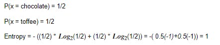
Assume, we replaced 15 chocolates with toffee. Now we have chocolates and toffee in the basket.

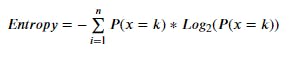
{where n denotes the maximum number of unique target variables}

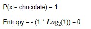
To find Entropy for our example :-

Case 1 - When we have 30 chocolates in the basket

Case 2 - When we have 15 chocolates and 15 toffees in the basket

The lesser the Entropy the better it is.

2. Information Gain

Information Gain measures the reduction in Entropy. It gives us the attribute that need to be decesion node ( root node or internal node).

We will choose that attribute whose Information Gain will be maximum. This solves our question, how to find the best attribute.

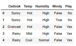
Lets create a sample dataset to apply Decision Trees algorithm. We are creating a dummy Weather data having target variable as Play.

Select the split with the highest value of Information Gain

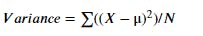
3. Gini Impurity

Gini impurity measures the impurity of the nodes and calculated as

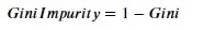
Where Gini is the sum of square probability of success of each class and measured as

Select the split with the lowest value of Gini Impurity

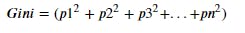
4. Reduction In Variance

Reduction in Variance method comes in use when the target variable is continuous. We take help of variance to split the node into child node in regression problems.

Select the split with the lowest variance

Now we will see how can we find information gain to find the feature for best split. Lets create a dummy dataset first.

# importing pandas
import pandas as pd

# creating dataframe
data= pd.DataFrame({"Outlook":["Sunny","Sunny","Overcast","Rainy","Rainy","Rainy","Overcast","Sunny","Sunny",
                               "Rainy","Sunny","Overcast","Overcast","Rainy"],
                    "Temp":["Hot","Hot","Hot","Mild","Cool","Cool","Cool","Mild","Cool","Mild","Mild","Mild",
                            "Hot","Mild"],
                    "Humidity":["High","High","High","High","Normal","Normal","Normal","High","Normal","Normal",
                                "Normal","High","Normal","High"],
                    "Windy":["False","True","False","False","False","True","True","False","False","False","True",
                             "True","False","True"],
                    "Play":["No","No","Yes","Yes","Yes","No","Yes","No","Yes","Yes","Yes","Yes","Yes","No"]})

data.head()

Output:-

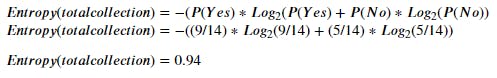
Step 1 - Compute the Entropy for entire dataset

We have 9 Yes and 5 No in our Target variable (i.e. "Play")

Step 2 - Which node to be selected as root node

For this we need o find out Entropy for each atributes. Lets start with "Outlook".

print("Sunny ->\n",data[data["Outlook"]=="Sunny"]["Play"].value_counts(),"\n")
print("Overcast ->\n",data[data["Outlook"]=="Overcast"]["Play"].value_counts(),"\n")
print("Rainy ->\n",data[data["Outlook"]=="Rainy"]["Play"].value_counts(),"\n")

Output:-

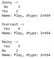
In Outlook we have 3 No, 2 Yes for "Sunny", 4 Yes for "Overcast", 3 Yes, 2 No for "Rainy".

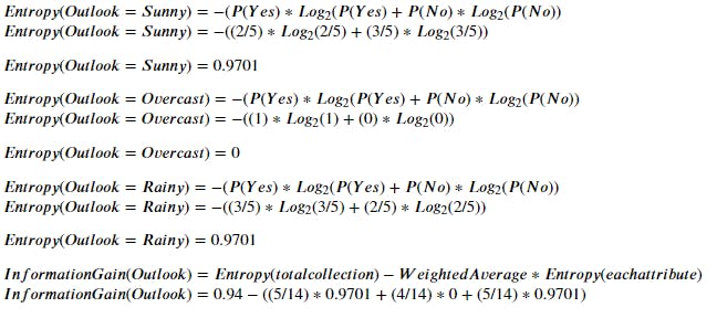
Information Gain(Outlook)=0.247

Similarly we will find Information Gain for rest of the attributes and will choose that attribute who has maximum Information Gain.

Model Development using Scikit-Learn

First import all the necessary libraries.

# importing libraries
import pandas as pd
import numpy as np
from sklearn.tree import DecisionTreeClassifier
from sklearn.model_selection import train_test_split
from sklearn import metrics

For the model development we are using iris dataset that is already available in sklearn datasets.

# import iris dataset
import sklearn
from sklearn.datasets import load_iris
iris= load_iris()

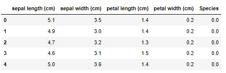
# making dataframe
iris_data = pd.DataFrame(data= np.c_[iris['data'], iris['target']],
                  columns= iris['feature_names'] + ['Species'])
iris_data.head()

Output:-

iris_data.describe()

Output:-

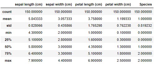
Now we will divide iris data into X ( feature variables ) and y ( target variable ).

# Store feature columns in X
X= iris.data
# Store target vector in y
y= iris.target

Splitting the dataset into train and test in the ratio of 70:30.

# train test split
X_train,X_test,y_train,y_test = train_test_split(X,y,test_size=0.7,random_state=1)

Implementing the decision tree classification model.

# decision tree classifier
clf = DecisionTreeClassifier()
# fit our model
clf.fit(X_train, y_train)
# predict
y_train_pred= clf.predict(X_train)
y_test_pred= clf.predict(X_test)
print("Accuracy on training :", metrics.accuracy_score(y_train,y_train_pred))
print("Accuracy on testing :", metrics.accuracy_score(y_test,y_test_pred))

Output:-

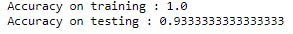
Clearly we can see our model has memorized all values of training data so it leads to Overfitting the training dataset.

# decision tree classifier
clf = DecisionTreeClassifier(max_depth =3, random_state = 42)
# fit our model
clf.fit(X_train, y_train)
# predict
y_train_pred= clf.predict(X_train)
y_test_pred= clf.predict(X_test)
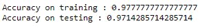
print("Accuracy on training :", metrics.accuracy_score(y_train,y_train_pred))
print("Accuracy on testing :", metrics.accuracy_score(y_test,y_test_pred))

Output:-

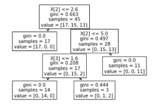
We can also check how our decision tree looks like using "plot_tree".

feature_columns=["sepal length (cm)","sepal width (cm)","petal length (cm)","petal width (cm)"]
sklearn.tree.plot_tree(clf);

Output:-

Advantages

1. Decision Tree is easy to understand, to ceate model and to explain to people.
2. There is no need to normalize as well as scale the data.
3. Decision tree can be used for both regression and classification problems.
4. Outliers and Missing values don't effect much decision tree model.

Disadvantages

1. Decision trees are prone to overfit the training data.
2. A small change in the data can give totally different tree structure.
3. Decision Tree are computationally expensive.
4. If continuous features are used the tree may become quite large and hence less interpretable.

You can check full code here.

Thanks for reading and please share your feedback.