


This tutorial is divided into three parts:-
- Eigen Value & Eigen Vector
- Singular Value Decomposition
- Application of Singular Value Decomposition
1. Eigen Value & Eigen Vector
If A as mxm matrix then a vector u (mx1) is called an eigen vector of A if
Au = λu
where λ is a scalar and called the eigen value of corresponding eigenvector.
# creating 2*2 metric
A= np.array([[1,2],[3,4]])
# finding eigen value & eigen vector of the metric
eigen_value,eigen_vector=np.linalg.eig(A)
#printing eigen value and eigen vector
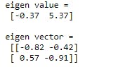
print("eigen value = \n",eigen_value.round(2))
print("\neigen vector = \n",eigen_vector.round(2))
Output:-
2. Singular value decomposition
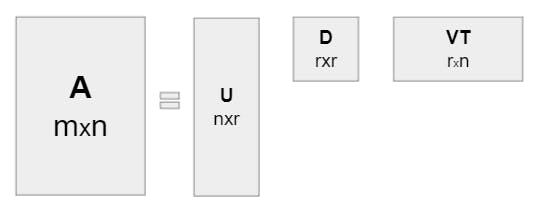
Singular value decomposition of A is the factorization of A into three different matrices such that
A = UDV^T ( V^T denotes transpose of V)
where U and V are orthonormal and D is a diagonal with positive real entries. Singular value decomposition is defined for both square and rectangle metrices.
Now we need to know how to find U, D & V. For this lets assume rank of A(mxn) is r. So non zero values of A is r. σ1 ≥σ2 ≥ σ3 ... ≥σn where σ(r+1) = σ(r+1) = ... = σ(n)=0, each σi is the square root of λi (i.e. eigenvalue of A^TA) and vi is the eigenvector corresponding to the eigenvalue.
V will be nxr matrix such that V = [v1 v2 v3 . . . vn] , each vi is of nx1.
D will be a diagonal matrix having diagonal elements as σ1,σ2,σ3,...,σr,...,σn where σ(r+1) = σ(r+1) = ... = σ(n)=0,
To find U , ui= Avi/ σi , 1≤i≤r so we get a set of r dimensional.
U = [u1 u2 u3 . . . ur]
Now lets understand this factorization using an example:
We are taking a 2x2 matrix for it.
# Lets create a 2x2 matrix
A = np.array([[17,4],[-2,26]])
print(A)
Output-

Finding Eigen value and Eigen vector of matrix A^TA
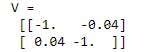
V is the eigen vector of A^TA matrix. We are sorting the eigen values and their eigen vector to decreasing order of eigen values
# Finding eigen value and eigen vector of A^TA
lambda_,V= np.linalg.eig(A.T@A)

# sorting in decreasing order
lambda_=np.sort(lambda_)[::-1]
# Defining 1st factor of matrix A as V
V=V[:, lambda_.argsort()[::-1]]
print("V = \n",V.round(2))
Output-
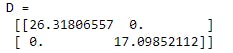
Finding Diagonal Matrix D
Elements of the diagonal matrix are square root of eigen values of A^TA.
# taking square root of eigenvalues of A^TA
sigma=np.sqrt(lambda_)
# Defining 2nd factor of matrix A as D
D = np.diag(sigma)
print("D = \n",D)
Output-
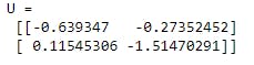
Finding U
# rank of matrix A
rank = len(sigma)
# Defining 3rd factor of matrix A as U
U = A@V[:,:rank]/sigma
print("U = \n",U)
Output -
Now we can verify by multiplying these factors that we are getting original matrix or not. We need to calculate UDV^T
# original matrix
print("A = \n",A)

# multiplying the factors that we generated
print("UDV^T = \n",U@D@V.T)
Output-
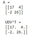
So we got our original matrix.
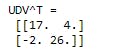
Generally we don't prefer that much calculation. We use inbuild function that numpy provides us.
# using inbuild function
U,D,VT = np.linalg.svd(A)
D=np.diag(D)
print("UDV^T = \n",U@D@VT)
Output-
3. Application of SVD
- Principal Component Analysis
- Compression Algorithm
Here we will discuss on Compression Algorithm. When we import any image than it stores as a large matrix where each element of the matrix denotes the pixel of the image. If the matrix is of nxn order than any transformation would require O(nn) which is computationally expensive. Instead if that we can send top k singular values of the matrix and right & left singular vectors ( U & V). This gives us O(kn) transformation. So we can get a low resloution of image that is sufficient. Lets look it as an example.
# setting the figuresize
plt.figure(figsize=(14,7))
# reading image
color_image=imread("Dog.jpg")
# changing image to 2d matrix
image=np.mean(color_image,-1)
img=plt.imshow(image)
# converting into gray
img.set_cmap('gray')
plt.show()
print("Image Size = ", image.shape)
Output-
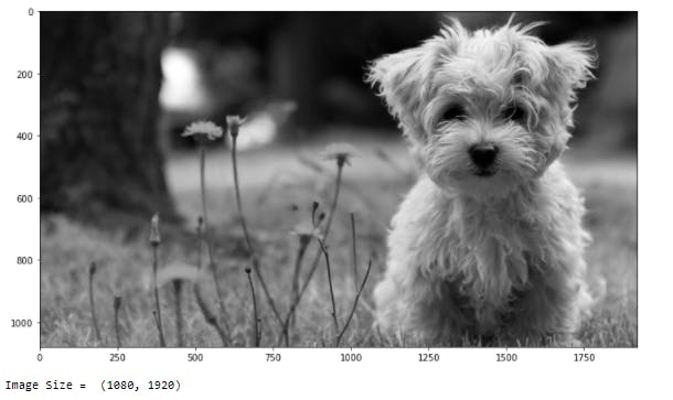
Now we have a image (matrix) of size (1080,1920). Lets find the factorization matrix U,D,V^T of the image.
# finding U,D,V^T using linalg.svd
U, D , VT = np.linalg.svd(image)
# converting D into Diagonal matrix
D= np.diag(D)
Now we will show our image for different rank selections and will check which image is suitable to use.
j=0
# plotting image for different different rank
for r in (10,20,40,80,100):
    # Generating new matrix using U,V &D which is approximate to original matrix (pic)
    Xapprox=U[:,:r]@D[:r,:r]@VT[:r,:]
    plt.figure(j+1)
    j=j+1
    img=plt.imshow(Xapprox)
    img.set_cmap('gray')
    plt.title("Rank = "+str(r))
    plt.show()
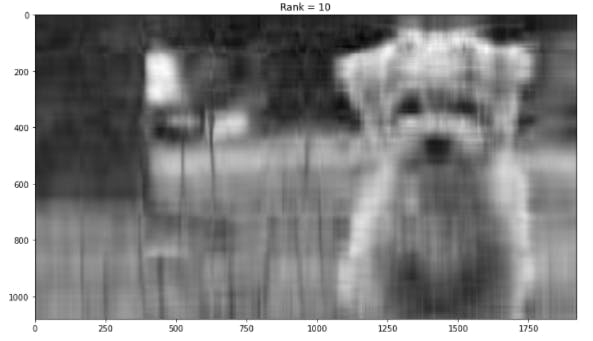
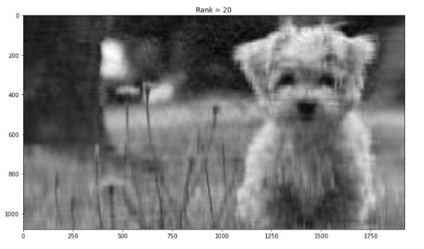
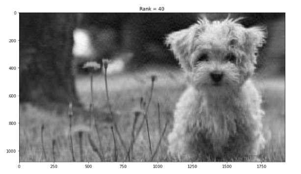
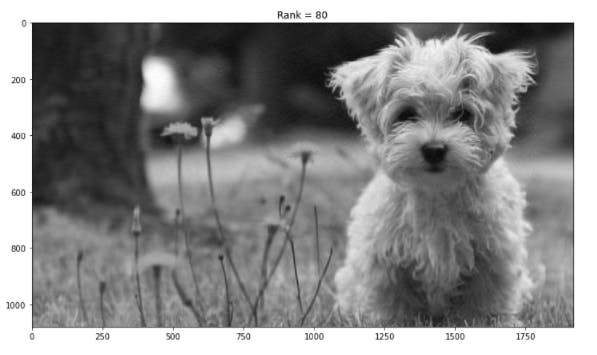

We can see that the last image where we are sending top 100 singular values give us clear image. Our original matrix has 1080x1920 = 2073600 values but in the last image we are using 100(1+1080+1920) = 300100 values which are roughly 15% of our original matrix. So we succeed to compress our image without loosing much information.
We can try it by taking different r values.
Also you can save your reduced image using 'imwrite'.
# importing imageio
import imageio

# saving reduced image
imageio.imwrite("SizeReduction.jpg",Xapprox)
Thanks for reading and please share your feedback.